Dispersion is a key concept in both statistics and optics, helping to illustrate how data points differ from each other.
It describes the degree to which data points in a set vary around a central value, highlighting the spread and variability present. Understanding dispersion is essential for analyzing data accurately, as it provides insight into how tightly or widely data points are clustered.
In statistics, measures of dispersion such as range, variance, and standard deviation quantify this variability. These measures reveal important information about a data set, like the consistency of measurements or trends within the data.
In the context of optics, dispersion can refer to how light spreads when it passes through different mediums, influencing how colors are seen.
Grasping the concept of dispersion allows for a better interpretation of both statistical data and phenomena in optics. By examining how data spreads, individuals can make more informed decisions and understand patterns that may not be apparent at first glance.
Fundamentals of Dispersion

Dispersion measures how data points differ from each other. It gives insight into the variability within a dataset.
Understanding dispersion is crucial for interpreting data correctly since it highlights the spread around central values like mean, median, or mode.
Defining Dispersion
Dispersion in statistics represents how spread out the values in a dataset are. It helps illustrate the degree of variability in the data.
Key measures of dispersion include:
- Range: This is the difference between the highest and lowest values in a dataset.
- Interquartile Range (IQR): This measures the middle 50% of the data, calculated by subtracting the first quartile (Q1) from the third quartile (Q3).
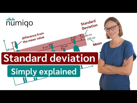
- Standard Deviation: It indicates the extent to which individual data points deviate from the mean.
These measures provide essential information for analyzing data distribution, helping to understand how consistent or variable the information is. For example, a low range or IQR indicates that the data points are closely packed, while a high range shows significant spread.
Comparing Dispersion to Central Tendency
Central tendency and dispersion are complementary concepts in statistics. While central tendency focuses on identifying a typical value through measures like the mean, median, and mode, dispersion reveals how much the data varies around these central values.
For instance, two datasets might have the same average (mean) yet differ widely in spread. One could be tightly clustered around the mean, while the other is more dispersed.
Understanding both aspects helps offer a complete picture of the data. By examining dispersion alongside central tendency, one can gain insights into the reliability of the central figure.
Measuring Dispersion

Dispersion shows how spread out data points are within a dataset. Various metrics help quantify this spread, providing insight into the variability and consistency of data.
Common Measures of Dispersion
There are several key measures of dispersion that analysts commonly use. These include:
-
Range: The difference between the highest and lowest data points. It is the most straightforward measure but can be sensitive to outliers.
-
Variance: This measures how much data points differ from the mean. It is calculated by averaging the squared differences from the mean. Variance may be calculated for a population or a sample.
-
Standard Deviation: The square root of variance, it indicates the average distance of data points from the mean. A low standard deviation means data points are close to the mean, while a high one indicates more spread.
-
Interquartile Range (IQR): This is the range between the first quartile (Q1) and the third quartile (Q3). It represents the middle 50% of data, offering a better measure of spread than the range, especially in datasets with outliers.
Calculating Dispersion Metrics
Calculating these metrics requires knowing some key data points.
For example, to find the mean or average, sum all data points and divide by the number of points.
To calculate variance:
- Find the mean.
- Subtract the mean from each data point and square the result.
- Average these squared differences.
For standard deviation, simply take the square root of the variance.
The interquartile range is calculated by finding Q3 and Q1 first. Subtract Q1 from Q3 to get the IQR.
Each measure of dispersion has its formulas and provides insights into the dataset’s variability, allowing for informed conclusions from data analysis.
Interpreting Dispersion Results

Dispersion results offer insights on the spread of data points in relation to a central value, such as the mean. Understanding these results can help readers grasp the variability within a data set and the implications of high or low dispersion.
Understanding Spread in Context
Dispersion measures how data points vary around the mean. Common metrics include the range, variance, and standard deviation.
The standard deviation is particularly useful, as it shows the average distance of each data point from the mean.
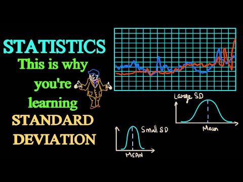
When data is tightly clustered around the mean, dispersion is low, indicating high precision in measurements. This is often seen in uniform data sets.
Conversely, high dispersion indicates that data points are widely spread out.
When evaluating data, it’s important to consider the context. For instance, a high dispersion in test scores may indicate significant differences in student performance, which could be linked to various external factors or teaching methods.
Implications of High and Low Dispersion
High dispersion can signal underlying issues, such as outliers or skewed distributions. An outlier may distort conclusions regarding average performance. In fields like finance or education, understanding variability aids in identifying risks and opportunities.
Low dispersion reflects consistency but may conceal important variations.
For example, in quality control, low variability in product measurements usually indicates effective processes. However, it could also suggest a lack of challenge, leading to complacency.
Thus, both high and low dispersion results provide critical insights into data behavior, helping analysts and decision-makers determine how to act based on the evidence at hand.
Practical Applications of Dispersion

Dispersion plays a crucial role in various fields, including statistics and optics. It helps understand how data values spread out in a dataset.
This is important for analyzing exam scores, where measures of dispersion like range and standard deviation can reveal student performance variability.
In statistics, the sample standard deviation measures how much individual scores deviate from their average. This can indicate whether a class performed consistently or had varied results.
Similarly, the population standard deviation applies this principle to an entire group, offering deeper insight into the overall performance.
In optics, dispersion is essential for applications like creating prisms and lenses. When light passes through a prism, it disperses into different colors. This phenomenon forms rainbows and enhances visual technologies.
Key Applications of Dispersion:
- Education: Understanding exam score variability aids in identifying students needing extra help.
- Optical Design: Engineers utilize dispersion principles to create high-quality lenses that minimize distortions.
- Data Analysis: Analysts employ measures of dispersion to interpret trends and patterns in large data sets.
In every application, recognizing how values spread or scatter contributes to better decision-making and innovations.

