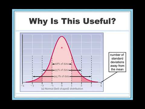
Dispersion plays a crucial role in both statistics and optics, providing insights into how data or light behaves in various situations.
Understanding the purpose of dispersion allows individuals to see how data points are spread out, revealing patterns that are essential for analysis and decision-making. In the context of data sets, measures of dispersion such as range, variance, and standard deviation help quantify the degree to which values differ from the average.
In optics, dispersion refers to how different wavelengths of light separate when passing through a medium. This separation produces phenomena like rainbows and the colorful edges seen in prisms.
By studying dispersion, researchers can gain deeper insights into the behavior of light, which is fundamental for advancements in technology, photography, and various scientific fields.
The knowledge of dispersion not only aids in statistical analyses but also enriches our understanding of light and color in the physical world. This exploration into dispersion highlights its importance across diverse applications, making it a fascinating topic worthy of deeper investigation.
Fundamentals of Dispersion

Dispersion describes how data points spread out in a dataset. Understanding key concepts like range, interquartile range, variance, and standard deviation is essential for grasping dispersion.
These measures help to analyze the variability in data, offering insight into the distribution of values.
Concepts of Range and Interquartile Range
The range is the simplest measure of dispersion. It is calculated by subtracting the smallest value in a dataset from the largest value. For example, if the values are 3 and 15, the range is 15 – 3 = 12.
The interquartile range (IQR) is more informative as it focuses on the middle 50% of data. It is calculated using the first quartile (Q1) and third quartile (Q3). The formula is IQR = Q3 – Q1. This method reduces the influence of outliers, giving a clearer picture of data spread.
To understand quartiles:
- Q1 is the median of the lower half of the data.
- Q3 is the median of the upper half of the data.
Variance and Standard Deviation
Variance measures how far each number in a dataset is from the mean and is calculated by averaging the squared differences from the mean.
For a sample, the formula is:
[ \text{Variance} (s^2) = \frac{\sum (x_i – \bar{x})^2}{n – 1} ]
where ( x_i ) represents each data point, ( \bar{x} ) is the sample mean, and ( n ) is the number of observations.
Standard deviation (SD) is the square root of variance. It provides a more interpretable measure of spread. In simple terms, it tells how much the values typically differ from the mean.
For example, a low standard deviation means values are close to the mean, while a high SD indicates a wider spread.
These measures are crucial in understanding both population and sample distributions.
Measuring the Scale of Dispersion

Understanding how to measure the scale of dispersion is crucial for making sense of data variability. This section explores two major aspects: absolute versus relative measures and how coefficients can aid in comparisons.
Absolute vs Relative Measures
Absolute measures of dispersion provide direct numerical values indicating the spread of data. Examples include the mean absolute difference, which calculates the average of the absolute deviations from the mean. Another common measure is mean deviation, which reflects how much data varies from the average.
In contrast, relative measures of dispersion express the spread in relation to the data’s central tendency. The coefficient of variation is a key example, showing the ratio of the standard deviation to the mean, making it easier to compare the variability of different datasets.
Both types of measures serve unique purposes. Absolute measures give a clear numerical view, while relative measures offer context, helping to unearth differences across datasets.
Utilizing Coefficients for Comparison
When comparing different datasets, coefficients of dispersion can be highly informative. The coefficient of range measures the spread relative to the total range of the data, offering insights into variability without considering unit scales.
Another notable coefficient is the coefficient of quartile deviation. This value focuses on the middle 50% of data, enhancing the understanding of dispersion in specific contexts. Lastly, the quartile coefficient of dispersion compares the interquartile range to the median, providing a sense of how data is spread around a central value.
These coefficients not only help in calculating dispersion but also make it easier to compare datasets with different scales or measurement units.
Practical Applications and Considerations

Dispersion plays a significant role in various fields, including optics and data analysis. Understanding how it affects measurements and interpretations can enhance precision and lead to better results. The following sections delve into handling outliers and their impact on data characteristics.
Dealing With Outliers
Outliers can distort statistical analysis, leading to misleading conclusions. These extreme values can arise from measurement errors or true variability in the dataset.
For precise results, it is crucial to identify and assess these outliers.
Methods to Identify Outliers:
- Scatter Plots: Visual representation helps to spot values that stand apart from the rest.
- Summary Statistics: Measures like the median absolute deviation (MAD) and quartile deviation can assist in determining acceptable ranges for data.
When outliers are detected, decisions must be made on retaining or removing them. This choice can significantly affect the overall accuracy and reliability of insights derived from the dataset.
It is important to strike a balance between preserving valuable data and ensuring the integrity of results. Thus, understanding dispersion enhances the interpretation and quality of analysis.

